How an Active Harmonic Filter Cancels VFD Harmonics

The Question

What is an active harmonic filter actually injecting when a VFD creates harmonic current?

It is tempting to picture the AHF producing an opposite copy of the complete VFD current waveform. That is not the right model. In the simplified case examined here, the utility/source voltage is approximately sinusoidal, the VFD is a nonlinear load, and the source still supplies the fundamental load current.

The AHF is connected in parallel. It measures the current, separates the components it is configured to address, and injects compensating current intended to oppose selected harmonic components. At the point of common coupling (PCC), the simplified current relationship is:

i_{source}(t)=i_{VFD}(t)+i_{AHF}(t)

(1)

Because the AHF harmonic current is opposite in phase to the targeted VFD harmonic current, less of that harmonic current flows upstream. The source sees the residual, not an idealized zero-distortion waveform.

The Simple Example

The fundamental current is fixed at 100 A so the harmonic arithmetic is easy to follow. Before compensation, the example VFD contributes 18 A of 5th harmonic current, 10 A of 7th, and 5 A of 11th.

At the maximum example command, the AHF injects −15 A at the 5th, −8 A at the 7th, and −4 A at the 11th. The minus signs describe phase opposition relative to the corresponding VFD harmonics; they do not indicate that the AHF is returning the entire load current.

Table 1. Selected harmonic-current components in the conceptual example

Component	VFD Current	AHF Current at Maximum Example Command	Remaining at PCC
Fundamental	100 A	Not cancelled in this example	100 A
5th harmonic	18 A	−15 A	3 A
7th harmonic	10 A	−8 A	2 A
11th harmonic	5 A	−4 A	1 A

For current total harmonic distortion, the individual harmonic RMS values are combined by root-sum-square and divided by the fundamental current:

THD_i=\frac{\sqrt{I_2^2+I_3^2+\cdots+I_n^2}}{I_1}\times100\%

(2)

This calculation includes only the 5th, 7th, and 11th harmonics because those are the deliberately selected components in the teaching example. A real spectrum can contain additional orders and interharmonics.

Step 1 — The VFD Current

A conventional VFD input stage draws current from the AC system in pulses rather than in exact proportion to the instantaneous voltage. The result is a nonsinusoidal input-current waveform containing the fundamental plus harmonic components.

The precise waveform depends on the drive topology, loading, line impedance, any AC or DC reactors, and other system conditions. We do not need a full rectifier analysis to understand the key point: the VFD behaves as a nonlinear load, so its input current is distorted even when the source voltage is approximately sinusoidal.

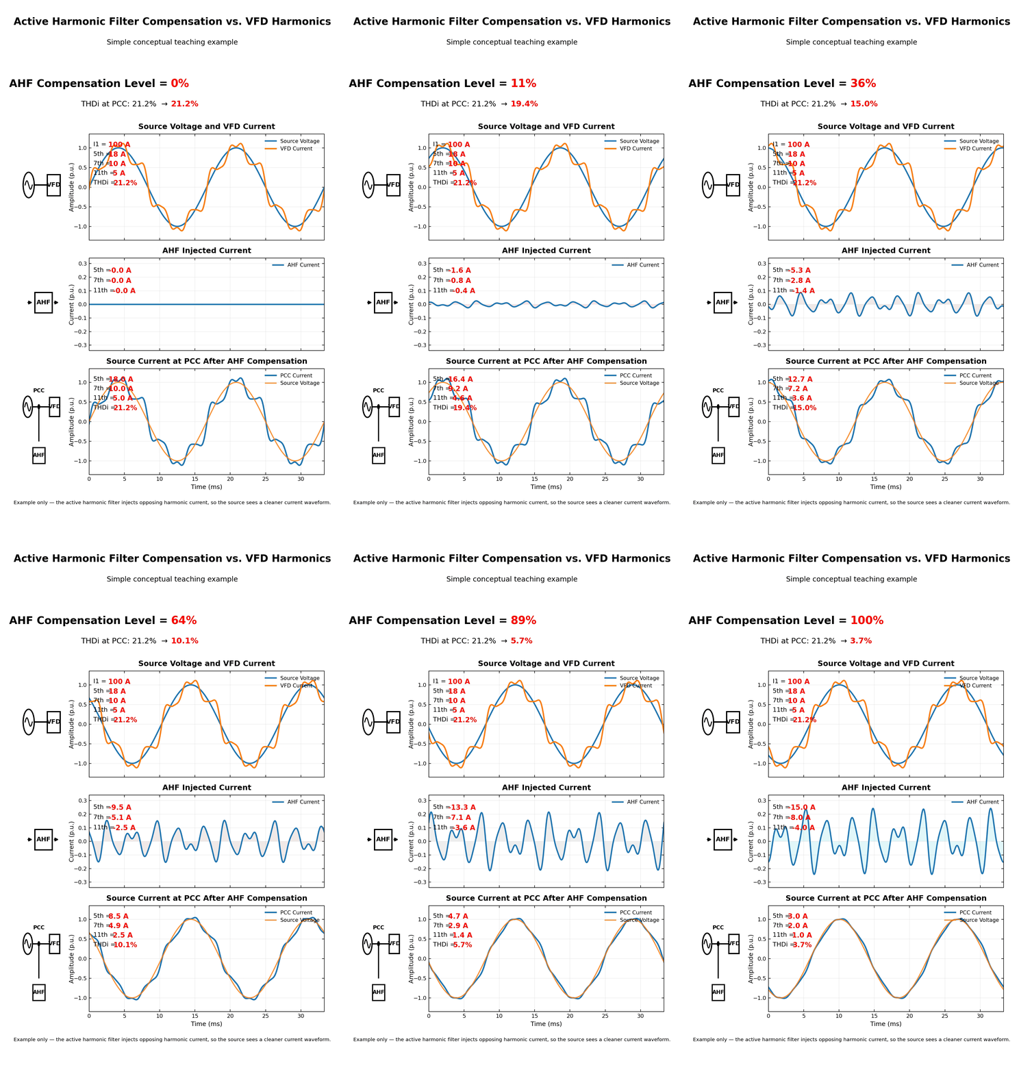
In the upper waveform of the animation, the orange VFD-current trace departs from the blue source-voltage reference. With no AHF contribution, all three selected harmonic currents flow upstream.

The initial distortion is:

THD_{i,VFD}=\frac{\sqrt{18^2+10^2+5^2}}{100}\times100\%=21.2\%

(3)

This 21.2% result belongs only to the stated numbers. It is not a generic THDi value for every VFD.

Step 2 — What the AHF Injects

The AHF uses current transformers (CTs) to observe load current or source current, depending on the product and whether the control arrangement is open-loop or closed-loop. The controller analyzes the measured waveform, determines the harmonic components to be addressed, and commands its power-electronic converter to produce compensating current.

For each selected harmonic order, compensation is a vector relationship involving magnitude and phase. In this simplified example, the injected component is shown with the opposite sign:

VFD 5th: +18 A; AHF 5th: −15 A
VFD 7th: +10 A; AHF 7th: −8 A
VFD 11th: +5 A; AHF 11th: −4 A

The AHF does not supply an opposite copy of the 100 A fundamental load current. It primarily injects the current components needed to oppose the selected harmonics, while the fundamental load current remains primarily supplied by the source.

Step 3 — What the Source Sees

At the PCC, currents sum. With the chosen phase convention, the maximum example command leaves:

\begin{aligned} I_{5,PCC}&=18A-15A=3A\\ I_{7,PCC}&=10A-8A=2A\\ I_{11,PCC}&=5A-4A=1A \end{aligned}

(4)

The residual THDi is therefore:

THD_{i,PCC}=\frac{\sqrt{3^2+2^2+1^2}}{100}\times100\%=3.7\%

(5)

The animation moves from 21.2% to 3.7% THDi as the injected example current increases. This is a conceptual interpolation between the stated endpoints, not a manufacturer performance curve or a claim that field performance changes linearly with a percentage command.

IEEE 519 applies harmonic voltage and current distortion objectives at the user PCC. That system-level PCC context is different from quoting the THDi of one drive or the output capability of one filter. This article uses “PCC” as the observation point immediately upstream of the illustrated load-and-filter connection; the actual project PCC must be defined by the system owner, utility, and applicable standard.

Why the AHF Current Does Not Look Like a Sine Wave

The middle waveform in the animation looks irregular by design. It is built largely from harmonic components rather than from the 60 Hz fundamental.

Adding several sinusoids of different frequencies and phases produces a composite waveform that is not sinusoidal. Here, the AHF current contains opposing 5th, 7th, and 11th components. That deliberately distorted injection combines with the distorted VFD current so the current upstream is closer to a sine wave.

This is the useful mental model:

A distorted load current plus a deliberately shaped compensating current can produce a less-distorted source current.

The AHF waveform should not be judged by whether it looks clean on its own. Its purpose is to produce the required change at the selected measurement point.

AHF Rating vs Load Current

An AHF is generally selected around the required compensation current and harmonic spectrum, not simply matched one-for-one to VFD full-load current. In this example, the root-sum-square of the commanded harmonic components is about 17.5 A, while the fundamental load current is 100 A. That observation illustrates the distinction; it is not a sizing shortcut.

Real selection must account for the measured or predicted spectrum, simultaneous nonlinear loads, desired residual levels, voltage, current derating, installation environment, CT arrangement, and any capacity reserved for other functions. Manufacturer selection tools may also account for harmonic diversity and the filter’s order-dependent capability.

Some commercial AHFs can use available current capacity for reactive-power compensation or load balancing. Those functions are outside this example, and they can compete with harmonic compensation for finite converter current.

What the Animation Simplifies

The visual isolates harmonic-current cancellation so the current paths are easy to see. It assumes:

fixed 5th, 7th, and 11th harmonic orders and magnitudes,
phase opposition between the selected load and AHF harmonic components,
healthy, approximately sinusoidal source voltage,
no background harmonics from other loads,
no change caused by source impedance,
no converter switching ripple,
no CT error or control delay,
and no manufacturer-specific sensing or control algorithm.

Actual load current changes with torque, speed, DC-bus conditions, front-end topology, line reactors, and supply conditions. The AHF has finite bandwidth and current capacity. Compensation can be very effective, but it is neither mathematically perfect nor identical in every application.

Practical Design Checks

Before selecting or commissioning an AHF, check the complete electrical system:

CT location and polarity: confirm that the controller sees the intended load or source current, with the manufacturer-required ratio, orientation, and phase assignment.
PCC definition: identify where harmonic performance will be evaluated; drive terminals, a plant bus, and the utility PCC are not interchangeable.
Harmonic spectrum: use measurements or credible study data across normal, minimum, and maximum operating states.
Source impedance: include transformers, generators, cables, and operating configurations that can change voltage distortion and system response.
AHF current rating: allow for the required harmonic compensation, order-dependent capability, load diversity, and any simultaneous correction functions.
Voltage rating: verify nominal voltage, tolerance, frequency, and grounding-system compatibility.
Enclosure and thermal derating: check ambient temperature, elevation, ventilation, contamination, and enclosure requirements.
Multiple nonlinear loads: consider aggregation and cancellation between loads rather than simply adding every nameplate current.
Background voltage distortion: establish what is already present before assigning all observed distortion to the local VFDs.

Commissioning should verify CT polarity and phase mapping, the defined control mode, available capacity, individual harmonic trends, and current distortion at the actual evaluation point. Compare results across representative operating states rather than at one convenient snapshot.

Key Takeaway

The VFD creates harmonic current. The parallel AHF injects current components intended to oppose selected harmonics. The upstream source sees the residual:

i_{source}(t)=i_{VFD}(t)+i_{AHF}(t)

(6)

In this teaching example, 18 A, 10 A, and 5 A of selected VFD harmonics become 3 A, 2 A, and 1 A at the PCC, reducing the calculated THDi from 21.2% to 3.7% while the source continues to supply the 100 A fundamental current.

That is the central idea—not that an AHF erases every harmonic, but that it dynamically supplies compensating current so less targeted harmonic current flows upstream.

References

IEEE Std 519-2022, IEEE Standard for Harmonic Control in Electric Power Systems — harmonic voltage and current distortion objectives and point-of-common-coupling context.
ABB, Technical Guide No. 6: Guide to Harmonics with AC Drives — nonlinear drive loads, harmonic spectra, and the external active-filter current relationship.
ABB Review, Actively Improving Quality: ABB’s PQF Active Filter — parallel connection, CT arrangements, and harmonic-by-harmonic compensating-current control.
Schneider Electric, AccuSine+ User Manual — CT configuration, harmonic mitigation, parallel operation, and optional reactive-power and load-balancing modes.
Project-specific one-line diagrams, source data, harmonic measurements, CT details, and the selected manufacturer’s current-rating and derating guidance are required for final design.